german version
First Acoustic Camera
Funktionen
Hardware
Mikrophon-Arrays
Interferenzschaltungen
Software "Bio-Interface" (later "PSI-Tools")
Among many other things, the program was developed to provide a tool for calculating interference integrals from various sources. This includes projections and reconstructions, as well as spatial mapping, interference patterns, and various other effects in pulse-propagating networks, which were first theoretically discussed in the book *Neural Interference*.
It also had an interface to a multi-channel data recorder (8 channels, later 16 channels with 50 kS/s and 12 Bit ADC-card Win30-DS). This also enabled electrical (EEG/EMG) and acoustic recordings; see also the 1998 help file: (HLP). A 1996 help file is also still available: (HLP).

The program proved useful for simulating and testing a variety of complex questions that could not be answered definitively "mentally." Thus, we experienced one of the biggest surprises when blurry images in the integration loop of the I. reconstruction were broken down with breakpoints: The wave field of the reconstruction, which defied rational interpretation due to various contradictions, appeared in its fullest beauty: with backward (inward) running waves whose front was also directed inwards. (Even the author didn't possess enough imagination to picture this wave field.)

CD cover 6/1996
Bio-Interface, or from 1997 onwards PSI-Tools, was used for five years (from 1994 to 1999). This enabled many initial acoustic verifications. However, a user interface geared towards simulation experiments, growing problems with Borland-C under Microsoft Windows 95, and the departure of our 'bee' (Sabine Höfs, 1997) caused development to stagnate. With the arrival of the first USB camera (Logitech QuickCam, VGA) in 1998, we began working on a software program (NoiseImage) focused solely on acoustics, which replaced PSI tools as early as 1999.
floppy disc 5 1/4"
Unfortunately, with the release of NoiseImage, the functions for time inversion of channel data (time functions) and channel data synthesis were removed. PSI-Tools is still required to calculate interference projections. Another reason for the relaunch was the channel data format of PSI-Tools. Here, all channels were stored sequentially in the file, which becomes inefficient with file streaming. Furthermore, the first USB cameras came onto the market in 1998, which could no longer be integrated into PSI-Tools with its now outdated software environment.
Even though it is no longer possible to record data with PSI-Tools, it can still be used for simulation. Starting with a bitmap of black pixels on a white background, PSI-Tools can generate 2- to 16-channel time functions (channel data). To do this, you need to specify the source coordinates and the propagation velocity in the generator array.
The propagation velocity and coordinates also need to be specified for the detector array. Then you can calculate the interference integral. By default, this produces a (laterally correct) interference reconstruction. Pulses (time functions) can be specified in their form. In addition to the RMS value commonly used in acoustics, other algorithms can be set; see the Help file under "Detection Method".
PSI-Tools can invert the channels in the time-domain to calculate the corresponding (mirror-image) interference projection.
Since PSI-Tools only performs reconstructions of the type To calculate the function f(t+Τ), the channel data (time functions) had to be inverted in time, and then the time direction of the resulting film had to be inverted again.
For the first time, the relationship between time direction, wave field, and interference integral could be visualized. PSI-Tools thus opened access to a new physics of interference integrals, to a wave physics that is no longer hypothetical but can be visualized. More information can be found in the section "Image Mirroring by Time Inversion" Ch.16.
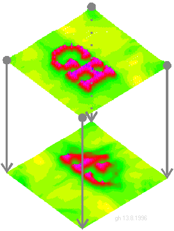
The image above shows a right-reading reconstruction of the type f(t+τ) and below shows a mirror-inverted projection of the type f(t-τ) from the same four time functions, which were time-inverted before the calculation began.
How else can this image be interpreted? Assume that waves travel at a finite speed from a red pixel in the upper image to the lower field. Then, at the point of intersection, an increased interference value is generated at the bottom. The color shifts towards red. This gives us a very basic understanding of image-forming communication in the nervous system. Because the system is overdetermined (4 channels, but 2-dimensional fields), the projection into the lower field will only be sharp near the axis.
For the reconstruction algorithm, see also the DAGA publication from 2007 as (PDF). Interestingly, until this publication, I was unaware of any beamforming book that didn't simply copy the incorrect formula for reconstruction of the type f(t-τ) from its predecessor. Only in the Transrapid (1993) and in a later DLR paper (1997) did the correct formula appear. Please forgive me for my continued dislike of the term "beamforming" to this day (2022): it encompasses much more: All these flawed books are surely still being used in student education.
A surprise awaits when you observe the corresponding wave field in image after image: In the mirror-inverted projection, it appears "natural" to us (the circular waves expand like water waves). But in the right-reading reconstruction, the waves run backward in time and they also have the wavefront on the inside. For more details, see both wave fields at this Link.
Note 2023: Now, 27 years have passed without many acoustics or brain researchers noticing this property of interference integrals. Or without theoretical investigations into it even being eligible for funding. Perhaps knowledge has become uninteresting?
Download PSI-Tools
PSI-Tools ran on IBM PCs (AT) under Windows 3.11, Windows 95, Windows 98, and Windows Me (all DOS-based). As of 2022, it was still possible to run it with limitations on Windows XP.
The ZIP file contains eight demonstration exercises (Demo 0 to 7) that allow you to test PSI-Tools. Demos 0 to 4 are described in the help file. There are some special considerations: Filenames must not exceed eight characters, and only uppercase letters (for saving the results) are permitted. PSI-Tools is quite slow; the algorithm was not yet optimized for speed. Demos 0 through 5 contain a generator bitmap from which channel data can be generated. As of 2020, all demo exercises could still be run under Windows XP. However, the path name must not be too long, and it doesn't work under 'My Documents' - PSI-Tools then reports "Incorrect parameter".
Help Files 1996, 1998 (Windows 95)
Short description of Demo 0 (see also PSI.HLP): In Demo 0, channel data is extracted from a generator array (bitmap "G"). Each black pixel of the "G" generates a Dirac pulse that arrives at channels 0...15 at different times.
Under "Parameters/Detector/Dimensions", you might want to increase the image resolution and calculate again. To calculate the corresponding (mirror-inverted) projection, invert the time axis using "Parameters/Channel filter/Reverse time" and execute it with "Actions/Channel to channel". Then recalculate. Caution: with 16 channels set, this is hopelessly overdetermined – it doesn't look good.
- Unpack psi.zip; Double-click PSI.EXE
- A warning message will appear: "Board not found" - this refers to the ADC card - click OK.
- Select "File/Load INI-file" and load it under DEMOS/DEMO0/DEMO0.INI
- Load "File/Load bitmap as virtual generator" under DEMOS/DEMO0/G.BMP
- Select "Actions/Picture to Channel" to synthesize time functions
- Select "Actions/Channel to Interference Integral": Hooray, it's calculating!
To set four channels: Set "Parameter/Generator/Number of Channels" to 4, and do the same for the Detector. Then change the channel coordinates with "Parameter/Generator/Channel origins," and do the same for the Detector array. Then save the INI file under a new name with "File/Save INI-file." Connections between the generator and detector arrays are considered latency-free. To view the result spherically, click "View/Pseudo3d window" ("3d-view window" is intended for volume calculations). You'll quickly notice that you need to change the pulse width (pulse sequence) and pulse interval (refractor time): the pulses are too jagged – it's best to change this in the INI file. Or just load Demo 2 (projection). Test: "Reverse time" will no longer be executed in 2022 - too bad! After this time reversal, the playback direction must also be inverted. A wave field will then appear, roughly in this form (Link).
GUI impressions
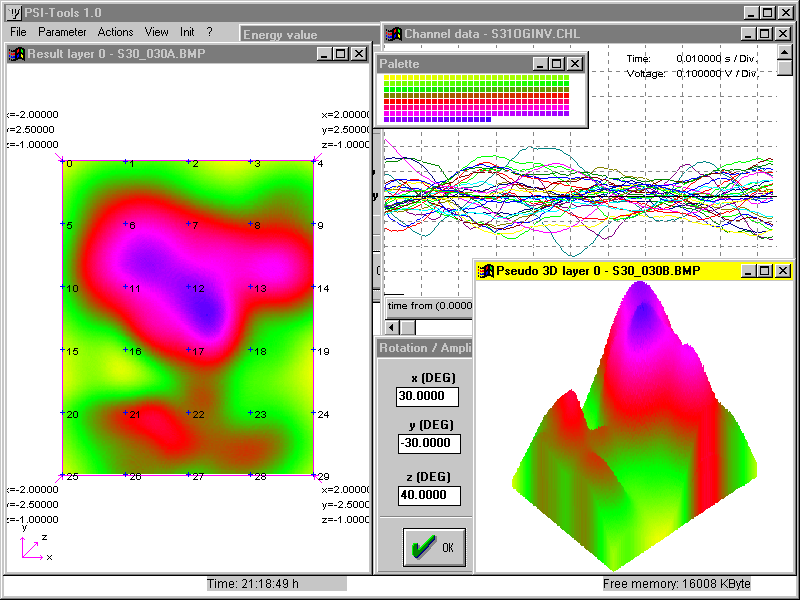
PSI-Tools surface: Interference integral of an Electrocorticogram (ECoG)
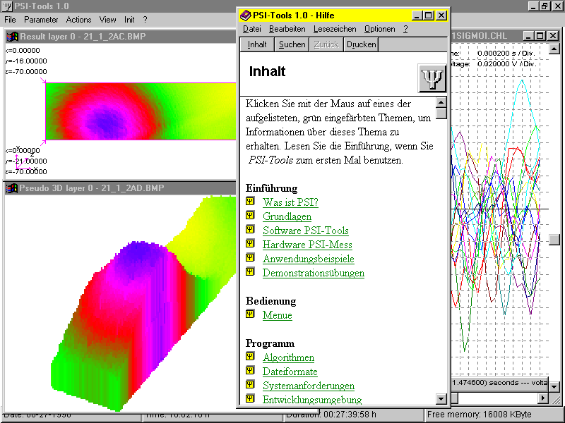
Acoustic image of a car crossing a street. Interference integral (interference reconstruction).
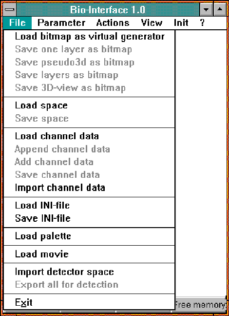
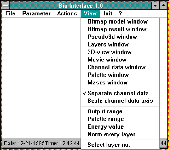
Menu Bio Interface
at Dec. 21, 1995 - before renaming "Bio-Interface" to "PSI-Tools".
File menu
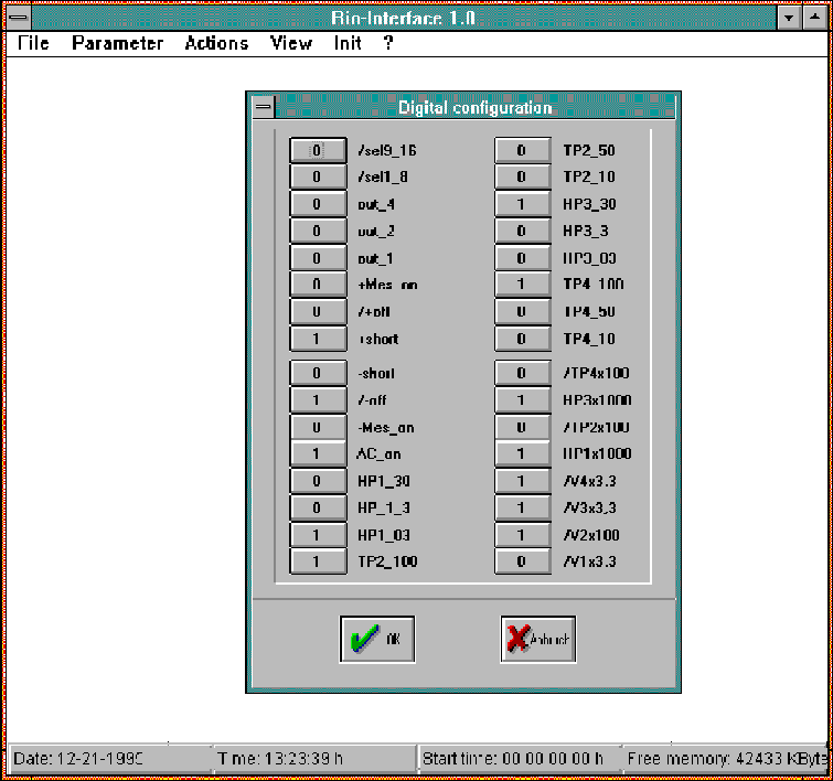
32 Bit preamplifier configuration menu (high and low pass filters). The Win30-DS-card had a 12-Bit ADC with low resolution. So filtering was done in hardware before AD-conversion.
Channel data synthesis menue to synthesize channels from a bitmap as generator space
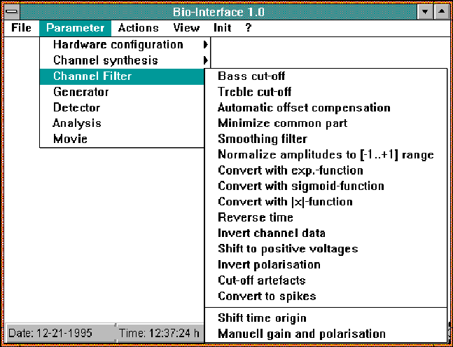
Digital filter possibilities with the option "Reverse time" to invert the time direction of all channels for interference projections
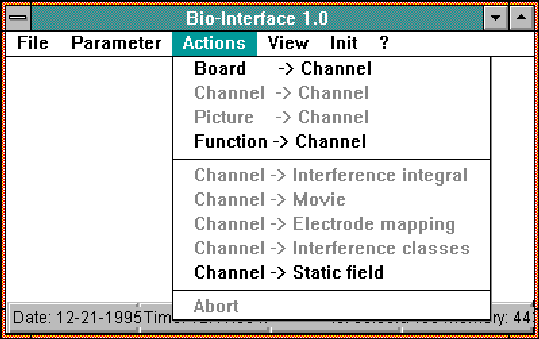
Actions menu. "Picture -> Channel" synthesizes channel data from a bitmap, shown as the generator field.
Views menue
Verifications Achieved
The following list shows that Bio-Interface (PSI Tools) became a key to understand interference networks. This enabled many (first) verifications of elementary interference circuits in simulation and measurement (acoustics):
1) Recovery of a low-channel excitation mapping as a pulse interference map from synthetic channel data (interference integral in the reconstruction) 8/94; First high-resolution reconstruction (300x300 pixels), GH 11/1994
2) Investigation of the influence of pulse parameters on the quality (sharpness) of an interference image (interference integral in the reconstruction, Sabine Höfs 8...11/1994)
3) Simulation of a neural mapping in an elementary interference circuit (interference integrals in the projection), GH 10/1996
4) Investigation of the influence of the axonal refractory time on the quality of an interference image (interference integrals, reconstruction), 10/94, GH 10/1996
5) Phantom excitation due to overexcitation caused by pulse intervals that are too short (e.g., due to insufficient refractoriness), GH 9/1994
6) Loss of an interference map due to overexcitation caused by insufficient pulse intervals (due to insufficient refractoriness), GH 9/1994
7) Fusion of widely separated, independent neuronal excitation maps into conjugate maps (interference integral, reconstruction), GH 10/1996
8) Movement of excitation maps due to (oppositely) varying channel delay times (moving) in the reconstruction, GH 9/94 - in the projection 9/1996
9) Zooming of excitation maps due to varying background velocity in the reconstruction 9/94, in the projection, GH 9/1996
10) Burst as a form of neuronal addressing, burst detection, and burst release. This was the first time that addressed neuronal multi-channel communication across single axons was simulated. ppN Neuronet Simulator (ppN Pulse Propagating Networks), GFaI/FHTW-FB3, Peter Puschmann, Gunnar Schoel, Gerd Heinz, October 18-20, 1994
11) First stationary sound image, GH 9/1994
12) First sound film, GH 8/1996
13) Discovery of an inward-propagating wave field in I-reconstruction f(t+T), Sabine Höfs and GH 5/1995
14) Detection of an outward-propagating wave field in I-projection f(t-T), GH 5/1996
Various evidence has only been presented in lectures. Rejected papers due to a lack of reviewers on the subject prevented a rapid dissemination of knowledge. Despite all the obstacles, the evidence has contributed to a new perspective on biology-oriented computer science, such as wave propagation in and outside of channel systems.
Acknowledgements
I would especially like to thank those who actively contributed to the development of this new field of knowledge. My particular thanks go to team members Sabine Höfs and Carsten Busch for their dedication to the development of software and hardware. Thanks also to the Managing Director of the GFaI, Dr. Hagen Tiedtke, and the Chairman of the Board of the GFaI, Prof. Dr. Alfred Iwainsky, for their extensive help and consistently friendly support.
Many thanks for valuable information, assistance, and discussions to Prof. Dr. Peter Bartsch (Charité Berlin, Institute of Physiology) and Dr. Hartmut Krüger (now Herzberge Hospital Berlin, Epilepsy Center).
My special thanks go to Dr. Torsten Griepentrog (Teupitz State Hospital), with whose help the thumb experiment (PDF) was successfully conducted on December 16, 1992, marking the beginning of this development.
Thanks also go to Prof. Dr. Langhorst and Dr. Manfred Lambertz (FU Berlin, Institute of Physiology), as well as to Prof. Dr. Thanks to Vogel (Charité, Neurosurgery) and Dr. Woichiechowsky for their expert advice. Thanks also to Prof. Dr. My thanks go to Raúl Rojas (Martin Luther University Halle/Free University of Berlin) for helpful discussions, and to Peter Puschmann and Gunnar Schoel (Berlin University of Applied Sciences and Economics, Department 3) for the joint experiments demonstrating elementary neuronal functions with their PPN simulator "NeuroNet".
Finally, I would also like to thank my discussion partners and moral support during the birth of the theoretical foundations of "Neural Interference": Andreas Thun (iris GmbH), Prof. Dr. Horst Völz (Free University of Berlin/Technical University of Berlin), Prof. Dr. Christian Hamann (Berlin University of Applied Sciences), and Prof. Dr. Achim Sydow (GMD-FIRST Berlin).
Last but not least, thanks to my wife Gudrun, who endured the months while I was working on the book "Neural Interferences" [NI93] written at my own expense.
Gerd Karl Heinz
E-mail: info@gheinz.de
File created Jan 12, 1996;
with remarks from June 2018, Jan. 2022.
Better layout with additional links Jan. 2023
Translation to english with support by the Google-translator Nov. 2025Access no.
since Sept. 10, 1996