
"If theory were to wait for experience, it would never come about."
Friedrich von Hardenberg
(Note: The page originally only showed excerpts from Chapter 12 "Biology-related Modeling" of the book "Neuronal Interferences" (1993) [NI93]. Some pictures shown here also exist in the animations page)
1. Foreword
2. Thumb experiment
3. Dermatoms and somatotopy
4. Delay masks
4.1 Projection in self-interference
4.2 Code generation
4.3 Code detection
4.4 Data addressing
4.5 Neighborhood inhibition
4.6 Level generation
4.7 In summary
5. Pulse sequences (bursts)
6. Distance determination using echo
7. Locating a noise
8. Penfield's 'Homunculus'
9. Balancing a human skeleton
10. The visual system (chiasm opticum)
10.1 Our world model
11. Diseases of the nervous system
12. Increased Sensitivity of the hand
13. How an earthworm squirms
13.1 Concentrated rope ladder
13.2 Leg control of an insect
14. A Hearing Neuron
The circuits shown here as interference networks are not electrical networks, but rather nervous networks with extremely low conduction velocities. All lines are delay lines! The electrical node abstraction of a line is not valid here.
The nervous system is full of mirror-inverted maps. Maybe there is a reason for this?
If you think about projections in time-delaying networks, you quickly realize, that forward-running time (without tricks) can only provide mirror-inverted images. A look at some neuroanatomy textbooks showed the author in 1992 that the nervous system is full of mirror-inverted maps.
That was the motivation to make the thumb experiment in 1992 and immediately afterwards to write the book "Neuronal Interferences" within a few months in 1993.
The decisive question of how the nervous system can be identified is, how it is networked. How do we imagine a connection between different communicating units? Is it a direct connection like a line connecting bell button and bell ("bell wire model")? If we reduce this idea, it would mean that every neuron would have to be able to potentially connect to every other neuron (of a few billion) in a universally learning nerve network. Consequently, if it must be assumed that potentially every neuron must be able to communicate with everyone else, this means that every neuron must be connected to everyone else. This in turn has the consequence that all 100 billion neurons ring when a bell button (excited neuron) is pressed. Consequently, nerve systems cannot be described with bell wire models of any kind. But how then?
The neural network theory brought forth a new approach since the 1940s. Threshold logic ("Threshold Logic", Jan Lukasiewicz 1920/1922) gave rise to the idea of only (connecting or) exciting neurons if a threshold value is exceeded, which comes from the simultaneous firing of different neurons. At least small, homogeneous, clocked networks could be described with this idea.
However, the limits of these models are reached when code or noise processing is required, or when signals pass through channels (chiasma opticum, homunculus).
If we include spatial coordinates and delay times on all paths in a model, we arrive at interference networks. But how should communication take place? About interference integrals, of course, about the relative simultaneity of the arrival of pulses. Relative means that it doesn't matter when a pulse started somewhere. The only important thing is that it and its twin brothers arrive at a destination at the same time. Then the goal is uncertain: it is only defined by the simultaneity, by delays.
The railway network is suitable as a conceptual model. Train stations stand for neurons, routes for nerves, trains for pulses. May trains commimg from Magdeburg, Rostock, Leipzig or Dresden arrive at Berlin Central Station. If passengers will be able to transfer between the trains, it would be necessary for the trains to arrive in Berlin at exactly the same time. In order for trains to be able to arrive in Berlin at the same time, they have to start at different times from the places of departure, if we assume that they generally have different travel routes and times.
Places of high interference (local overlapping of many wave crests) require a very precise, spatio-temporal timing of the elementary waves involved. Pulses can come from anywhere. The wave front only have to arrive at the exact destination at the same time to meet other wave fronts. We suddenly conceive a nerve web as the most brilliant, decentralized machine in the universe. We also understand that interference networks are a group of complicated networks that have the property of associating several transmitting neurons with corresponding receiving neurons. And we understand that we are still at the very beginning of their knowledge. We will call networks that do this "projecting networks" or "interference networks".
The author was lucky enough to discover some of them.
After I realized in 1992 that nerves are supposed to conduct very slowly and that pulses must be the carriers of information, my first question was about the conductivity of biological material.
One of the first experiments was to examine a pork chop for electrical/ionic conductivity. A conduction velocity could not be determined because the available tube oscilloscope was too slow. The pork chop behaved like an RC equivalent circuit.
I got hold of books on neuroanatomy. On the one hand, I found the table of conduction velocities according to Erlanger/Gasser, and on the other hand, I met Dr. Torsten Griepentrog. Together we developed the thumb experiment.
If you are wondering why it is so difficult to obtain neural data, consider that the ionic conduction of flesh is many times better and faster than that of the wafer-thin nerve fibers hidden beneath it. Without the shielding ring below the thumb electrode, nothing would work; see photos of the measuring arrangement in Abb.7 of IWK94.
In fact, nerves were not designed by evolution to conduct signals quickly. On the contrary, they conduct signals extremely slowly compared to the material surrounding them!
If the thumb is electrically stimulated, the progressing impulse can be picked up on two non-invasive accessible nerve tracts (n. radialis and n. medianus) (NLG/EEG averager set at least 10 times; a shielding electrode is arranged between the stimulus electrode and the sensor electrodes).
A small change in the position of the thumb causes that the time difference between the arrival of both pulse parts varies by around 0.5 milliseconds. The wavefront of the impulse passes the sensor electrodes more or less obliquely. The picture even shows a sign reversal of the wavefront when the thumb is pointing inwards.
The right part of the picture shows mappings that vary with the position of the thumb on a hypothetical reception field.
Fig.1: Thumb experiment, G. Heinz, 1992, Source. It was the introductory experiment by the author, measured with an Electroencephalograph (EEG).
Stimulation of thumb by ring electrodes and recording of two nerves (N.radialis and N.medianus) shows the forthcoming of impulses in dependence of the position/location of the thumb. (Use a guard ring between thumb-electrode and sensor-electrodes to avoid artefacts. Averaging: 10-times minimum).
The EEG shows, that the immediately occurring electrical/ionic conduction, despite the shielding ring, is many times stronger than the signals recorded from the radial and median nerves. A usable signal is only obtained with an averager.
As we will see in the discussion of Hebbian learning, it is assumed that the tiny electric fields emitted by axons represent the starting point for Hebb's rule to function and for a dendritic growth process to begin.
If the thumb position changes, the delay-difference between the sensor electrodes changes too. The wavefront passes more or less diagonally over the sensor electrodes.
If we suppose, that elsewhere in the body (medulla spinalis, ganglion spinalis...) lay neurones in a circuit in a real distance (s), we can calculate the properties of this interference network with real velocities. Interference networks can also be fast - but only on the myelinized transmission wires (r, m).
This simple interference network showed parts of a mirrored projection (red to red, blue to blue), (Measurement from December 16th, 1992, Landesklinik Teupitz; Dr. Gerd Heinz with Dr. Torsten Griepentrog). So Christmas 1992 became the most sleepless celebration of my life. Now the thoughts "only" had to be sorted and written down. The book "Neuronal Interferences" was essentially written within 3 months.
The first publication of the thumb experiment was in the IWK article "Relativität elektrischer Impulsausbreitung als Schlüssel zur Informatik biologischer Systeme. 39.IWK Ilmenau (PDF, german), (HTML, german) translation (HTML, english).
See further details in the web-publication "Beobachtbare Relativität neuronaler Impulsausbreitung - Ein Versuch mit Konsequenzen für die Neuroinformatik" (PDF german).
3. Interference network - dermatome - somatotopic areas - projection trajectories
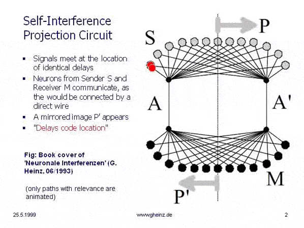
Fig.2: Communication principle of a nervous interference network
This simplest, monomedial interference circle is on the cover image of the manuscript Neuronal Interferences (1993). A sending space interferes with a receiving space via axons A and A'. Neuron P should send a pulse into the network. At the point P', where both pulses arrive at the same time, an above-average value of the interference integral arises; there is simultaneity there and only there does new excitation arise. Similar to an optical lens projection, a mirror image of the sending room is created in the receiving room - an optical projection is created.
If you imagine the rooms to be larger, you would see that the drawing can represent all the projection pathways of the nervous system - both ascending and descending.
It is noteworthy that excitation from the location P to a location P' can only ever be passed on in a mirror image - an image template P becomes a mirror image P' - as in optics. The animation (behind the image) makes it clear that transmission and reception locations in the interference model are defined solely by the delays of the connecting network - but not by the type of cabling and not by the strength of weights (Hebbian law).
A crossing is no more necessary in the optic nerve than in the pyramidal tract. They can be present, but have little influence on the type of images created.
A special feature of all interference images is their coherent (tear-resistant) projection, see for example a simulation of superimposed interference maps in nervous parameterization.
Only reflective, somatotopic images of this type are known from the nervous system. The so-called fiber exchange is known from the dermatome: A dermatome is always innervated by several nerve bundles.
Even an autonomous region is not autonomous. It shows a superposition of different nerve fibers in at least one direction. All of these are very clear indications of the function of the nervous system as an interference network: The nerve network can only be understood and calculated in terms of interference.
4. Delay mask and dynamic elementary functions of a neuron
If we accept the real existence of low conduction velocities, finite transit times and geometrically (λ = v·t) short pulse needles in nerve networks and if we accept the possibility of multiple parallel transmission of pulses, then we also have to acknowledge, that communication between two neurons becomes more efficient, the more precise incoming partial waves meet (interfere with each other).
The selectivity of a neuron has something to do with an extremely precise coordinated runtime architecture:
In order for Hebbian weights to be learnable at all, the delays must be correct, and a cleanly coordinated interference network must exist so that the neuron in question can be addressed at all.
For example, a partial delay can be tuned to the maximum excitation of the neuron via the thickness and length of a fiber.
But how can we grasp these things mathematically?
Let us consider a most elementary connection network consisting of two neurons and a few delaying fibers. First, we want to transport a simple pulse between both neurons with maximum efficiency.
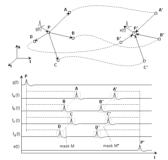
Fig.3: Simplest interference network
We split the structure into three parts:
The delays PA...PD should be assigned to a pulse-generating neuron; in the matrix representation we call these delays delay vector or mask
M = {PA, PB, PC, PD}.Delays AA'...DD' should cover the transmission path with a delay vector
L= {AA', BB', CC', DD'}.Delays A'P'...D'P' should be sent to the receiving neuron with the mask
M'= {A'P', B'P', C'P', D'P'}.Of course, a certain amount of time passes during the process τ = {PP'};
in vector notation T = τ · {1} ({1} is the identity-matrix).
For example, if we multiply the time functions in P' sample by sample (convolution), then it quickly becomes clear that the running times of the individual paths must be identical if we do not want to get a time function made up of zeros, if one of the time functions becomes zero:
(1) PA + AA' + A'P' = PB + BB' + B'P' = ... = PD + DD' + D'P'
in vector notation then applies:
(2) M + L + M' = T (mapping condition)
Consequently, the three masks are inextricably linked.
4.1 Projection in self-interference
The receiving neuron only receives the input time function identically at the output if its delay mask fulfills the condition from (2).
(3) M' = T - M - L (with T = const.)
Neuron P' is only maximally excited by P if it has formed a suitable delay mask M'.
If the mask M does not fulfill condition (3), the inequality applies
(4) M' ≠ T - M - L
and if we assume additive linkage with a suitable threshold value in OR form, a single pulse at the input generates a pulse train at the output. Neurologists call such short pulse sequences "bursts".
If the bias is chosen very high (multiplicative AND type), the circuit does not react to individual pulses. Instead, it detects a pulse group with the delay mask M', see Bursts.
If we find nerve cells whose delay vectors correspond to the formula
(5) M + L + M' = const. = T
with T = τ · {1}
({1} is the identity matrix )
then one sends out a burst y(t), that only the other can receive and which it converts back into a single pulse z(t). If several nerve cells, which have different delay vectors, send on a common transmission line, and there are nerve cells on the receiving side, each of which can only select a specific burst, then we find a transmission principle that can explain the transmission of different data streams on a common line.
The principle should be called 'data addressing'. At the moment this principle is purely hypothetical. But since it could be demonstrated comparably easily (with just one electrode), we can have hope.
See also a more detailed description of neighborhood inhibition in Ch.18 of the "Second Informatics".
The same principle prevents excitation from jumping between neighboring neurons. If incrementally very closely spaced neurons have connection points and identical structure, they have nearly the same delay vector M.
Since M + 0 + M' = T must be fulfilled for addressing (L = 0 disappears) and therefore M' = T - M applies, but the geometric structure demands M' = M, there is only one (stupid) solution for M and M' (besides the trivial solution zero):
(6) M' = M = T/2 = τ/2 {1},
which, in the roughest approximation, means that the coupling synapses of both neurons must be arranged in a circle around the soma in a radius
r = v · τ/2 (with conduction velocity v). We assume that the soma of the neurons overlay each other.
The principle thus explains a dynamic neighborhood inhibition on the basis of delays (independent of, for example, inhibitory synapses). One could say that, due to their dynamic nature, excitation does not jump between two neurons connected at the same location nodes - which seems to be an extremely advantageous property of nerve networks.
This principle ultimately prevents the unintended jumping of excitation between neighboring neurons and the total breakdown of all information transmission.
To produce control potentials for bias or other, we need a possibility for level generation. If the detecting neuron has an integrating property, a detected burst can lead to an increase in potential. We call this property level generation. If the integrating effect is strong enough, sliding background potentials can be created in this way, which in turn are needed to control zoom or movement. It can be assumed that we measure exactly these control potentials in the EEG. Own EEG experiments (see there) showed insufficient interference reconstructibility, this would fit with this.
See also Ch.8b, p.191 and Ch.10, p.212 in NI93. Level generation could be verified in the simulation with the simulator 'Neuronet' at the FHTW Berlin on October 20, 1994 (Peter Puschmann, Gunnar Schoel, Gerd Heinz), see VirEx96, 17th experiment, p.17.
The result are laws, that can be viewed in a certain way as an extension of McCulloch/Pitts to include Hebb's rule and Jeffress interference network.
We can observe dynamic, elementary, neuronal functions:
Code generation Code detection Data addressing Neighborhood inhibition Level generation
These certain properties are discussed for the first time in the manuscript [NI93]. Building on this, complex properties of interference networks can be explored. The most important are:
Zooming of an image when the propagation speed changes Moving the image if the delay changes in the transmission channels in the opposite direction Conjugation: merging superposition of images in a detector field Interference overflow with strong firing or too short refractoriness of the axons
Fig.4: Burst generation and burst detection
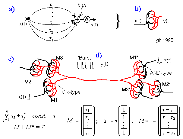
Fig.5: Burst model example. a) Equivalent circuit of a coupling point; b) connected neurons; c) Example connection of several neurons; d) generated burst.
About the function: Neurons 1 to 3 may have different masks (delay vectors) M1 to M3. For this purpose, pairwise inverse vectors M1* to M3* may exist. Then (apart from possible permutations not considered) the excitation generally jumps only from M1 to M1*, from M2 to M2* and from M3 on M3* via and visa versa.
Going beyond the synaptic, neuronal coupling, which is the subject of neurocomputing, temporal relations play a crucial role in pulse-like signal propagation in the nervous system. The simultaneity of the arrival of impulses determines the excitability of a neuron.
We discover that new, basic neuronal functions can only emerge by paying attention to delay times (see also [NI93]). Millions of years before time division multiplexing (TDM) was invented by humans, nature had already invented bursts as a stochastic multiplexing method:
At M1, M2 and M3 (Figure 5c) bell buttons can now be connected, while bells can be connected to M1*, M2* and M3*. For example, if M1 is pressed, it only rings at M1* etc..
6. Measurment of Distances by Echo
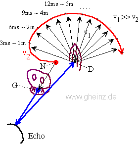
Fig.6: Simplified interference circuit to measure any distance by echos.
A generator neuron N emittes an excitement that moves on two paths: one part is transformed into sound by the voice, the other part (red) walks slowly with speed v2 radial around the noise sensor (ear D).
In the moment the echo arrives the ear D, an excitement expands with higher speed v1 circular from D. Then the interference location correlates with the distance of the echo-reflecting object. We get a map of the outside echos along the radial fibres.
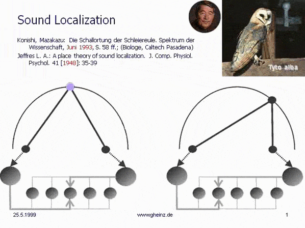
Fig.7: Lloyd A. Jeffress model for noise localisation 1948, simplified by Mark Konishi* 1993.
Historical this was the first attempt for an intermediale, projective interference network. Note, that the generating input map excites mirrored the detector field - the neural network. A more right-hand noise location interferes to a more left-hand neural excitement and visa versa. The projection appears mirror-inverted.
*Konishi, M.: Listening with two ears. Scientific American (April 1993), p. 66-73
8. Mirror-inverted body projections in the spinal cord - Penfields
'Homunculus' as a hyperbolic interference circuit
Compared to interpretations of the gray matter in the vertebral bodies of the spinal cord for generating reflexes (cf. Duus, P.: Neurological Topical Diagnostics, p. 10ff.), the hyperbolic arrangement of unmyelinated gray matter in the spinal cord suggests to the circuit engineer that delay times must play a dominant role. The question is, for what purpose?
An interference network provides physically relevant evidence for the generation and development of mirror-image body projections to/from the cortex. As the thumb experiment shows, the delay times of stretched or compressed nerve fibres vary, when they were stretched or compressed.
Let's assume, that a nerve network has purely functional assignments via bell wires. Why do we need then interconnected maps like the Homunculus? These would actually be superfluous, if there wasn't a very special problem that only becomes apparent through interferential observation.
Let us further assume, that a doorbell model between the brain and the body would require so many axons, how sensors and actors are present. They would not fit through the spinal canal. An interference model, on the other hand, saves axons because 'images' (mirror-inverted projections) can be transmitted through many fewer channels. The number of remaining axons decreases.
This is exactly where an interface problem arises: Every time, the head is tilted or rotated, the images of the body in the head would move and slip along with it - no data could be exchanged between the cortex and the body, because they interact. Every time the neck is stretched or the body is turned, they would be sent to a different location within the brain.
Imagine a slide projector that shines from the first into the second (and last) wagon of an littls train: with every curve and bump, the image in the rear shifts or disappears completely.
The thumb experiment in 1992 provided certainty that when the thumb is spread apart, interference-locations will also change, so the same can be expected from bending the spine.
The solution is ingeniously simple. Nature created a projection plane, that can be focused from both sides, from brain and from body (see Movement and Zooming). For our train, for example, this would be a screen that we stretch in the middle of the joint between the two wagons. Projections can now be focussed from both sides. Images (motor and sensory) no longer shift as much. But this model is only symbolic; in reality, things are different.
By varying the conduction speed of the glia in the cortex, images can be refocused on defined areas, despite movements.
The motor and sensory cortex, known as 'Homunculus' [Love & Webb 1992, p. 19] (see e.g. also Wikipedia), when viewed interferentially, forces the creation of a necessary coupling point between organs (cortex and body), which are movably connected to each other.
To get an idea of how nature solves this technical puzzle in the spinal cord, we look at the pathways and nerve cross-sections in the spines. If we mark the wave fronts of a pulse in red, green and blue, then the relationships shown can be found.
The basic idea of an hyperbolic interference circuit roughly creates mirror-inverted a height mapping of Penfield's Homunculus. Furthermore, it creates a (planar) mapping that expands the homunculus in the anterior/posterior direction when more than two axons can be assumed to be acting. It would be conceivable, that this plays a role in evolution or in individual genesis: a body without a neck would not need to develop a homunculus.
Gardner's 'reflex pathway' is interpreted as presented. What would be more suitable for the model, however, would be a bidirectional, both sensory and motor coupling into the spinal cord simultaneously from the front and from the back (c. dorsalis, c. ventralis) - without distinguishing between directions. An intermediate conversion in the spinal ganglion would not be functionally significant. However, it should be noted, that bilateral efferent and afferent coupling appears to be unknown so far. It still needs to be proven.
The well-known lateral reversal within the spinal medula is not relevant to the model. This reversal is generated by the model's own dynamics. A pulse originating from the right at C4 or S6 will appear in the left cortex, and vice versa.
The question of exactly which paths or pathways the impulses take to reach the cortex is also not relevant. What is relevant, however, is that all signals are delayed in the same way and that there is no additional change of sides in the nerve cord in the spinalis muscle. A physically real crossing of the pathways, as found in medical textbooks, would require a different model.
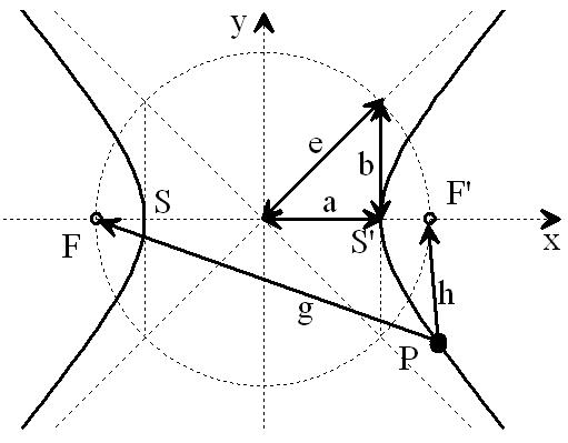
Figure 8a: Hyperbola from NI93, Chapter 3, p. 77 (with highlights). The vertex distance SS' = 2a = |g - h| determines the path or travel time difference of any point P on the hyperbola to its foci F and F'. The circle with diameter 2e characterizes the distance between the foci F, F'.
If the vertex distance 2a of the hyperbola is varied, the transit-time difference |g - h| of the new, corresponding hyperbola changes accordingly. Vertices SS' that are closer together are associated with a smaller transit-time difference, while those that are further apart are associated with a larger transit-time difference. See also the parametric plot image with plotted relative length differences on page 78 in [NI93] Ch.3.
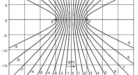
Figure 8b: Hyperbolic family from NI93, Chapter 3, p. 78. The path differences (g-h) correspond to the transit-time differences, mediated by the conduction velocity of the fibers.
If two signals from the same origin, one above and one below, enter the hyperbolic branch and meet at P, the signals can be transmitted to the foci with a new transit-time difference 2a = |g - h|. They can then be conducted towards the cortex via the adjacent white matter (myelinated fibers).
Extending this line of thought, body projections are created in the cortex, which are assigned to the fibers entering at the various vertebral bodies. One approach, for example, is to assume that the focal distance FF' = 2e is kept constant by varying the slope of the dashed tangents b = sqrt(|e² - a²|). But to refine this model, significantly more extensive investigations of the spinal medula would be necessary.
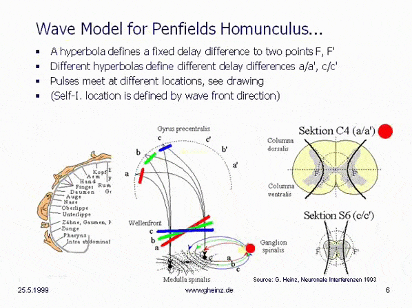
Fig.8c: Model of hyperbolic, mirror-inverted body projections over the spinal cord. Simplified model of the medulla spinalis. Source: Heinz, G.: [NI93], Ch.12, p.251-253. References: Schmidt, R.F., Thews, G.: Human Physiology. 24th edition, Springer-Verlag 1990, p. 105; and Rauber/Kopsch: Human Anatomy; Volume III: Nervous System, Sensory Organs. Georg Thieme Verlag Stuttgart, 1987, p. 299
If it is assumed, that the thickness of the spinal cord varies height-depending, a hyperbolic projection ([NI93] Ch.3, p.77 ff. and Homunculus [NI93] Ch.12, S.251 ff. requires a decreasing transit time difference with decreasing thickness of the spinal cord, compare section C4 (a/a') with section S6 (c/c'). (For better understanding see Wikipedia/ Hyperbola). This means, that the wave fronts (red, green, blue) head to different cortical interference locations. Assuming the same neuron properties, the transit time difference is smaller for slice S6 (c/c') than for slice C4 (a/a'). See also images of the Spinal cord in Wikipedia.
Because of a smaller transit time difference, a wave front shown in blue from S6 would inevitably rise to c or c'. While from C4 a more oblique wave would rise to a or a' because of a larger transit time difference. (The probability of excitation is maximum in the area in which the pulses arrive at the same time.) Thus, the anatomy inevitably produces a location assignment that corresponds to the motor and sensory area of Penfield's 'homunculus'.
This simplest interference model, which can be verified by runtime measurements, essentially generates the following properties:
The mirror-inverted body projection in the sensory and motor cortex The height assignment, typical for the Homunculus A decoupling of the excitation maps between cortex and body
What seems surprising, is the fact that both, the necessary connections at c. ventralis and c. dorsalis are present at the right place. What is even more surprising, however, is that even the gray matter of the medulla spinalis is arranged in exactly the right hyperbolic shape.
Section C4 gives the impression, that two hyperbolic adjustments are possible in the lower part. The evolutionary idea behind this is still unclear; it can be assumed, that the motor areas separate from the sensory areas; as is well known, these are located next to each other in the cortex parallel to the central groove.
It should be noted that this model, with only two upward-moving fibers, is extremely simplified. One would expect a significantly larger number of nerve fibers to be involved in the interaction.
Since neural networks are extremely sensitive to tiny changes in transit time or length, other interpretations are unlikely.
In the 1950s, Rosenblatts "Perceptron" was the first machine that could balance a single broomstick. If we now stand ten (small) broomsticks one on top of the other, we become aware of the theoretical impossibility that our upright walk entails.
Using control theory, it is probably not possible to balance an unstable tower consisting of ten joint parts so that it can stand stable. Control processes between the joints would reinforce each other; stability of the entire system can hardly be achieved with local control algorithms. So where can be found a solution?
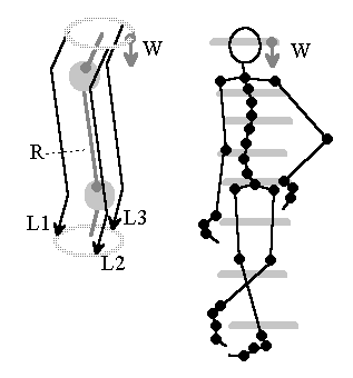
Fig.9: Model of a self-balancing skeleton. Source: [NI93], Kap.12, p.250
If we think about the thumb experiment, a virtual wavefront could help, running downwards from the vestibular system in the head, to which local muscle groups align themselves.
If it is assumed that at least three nerve fibers L1...L3 exist in indicated manner, a (virtual) wave can be used to stabilize the system. A periodic repetition of a wave front W running downwards from the vestibular organ on several nerve pathways is assumed, the wave gradient of which reflects the tilt of the vestibular organ. Local muscle groups could adjust according to their relative position that deviates from the wave front.
However, the simple model is missing further components: How can it be ensured that all skeletal muscle groups act with proportional forces? How can the system squat? Hard detailed work still needs to be done here.
The simple local algorithm for achieving global control is: each element must align its direction orthogonal to the wavefront direction, assuming the wavefront appears periodically.
10. The visual system (chiasm opticum)
Even in ancient times, the question was asked as to how the world, which appears mirrored on the retina, could be mirrored back. If the neurons between the retina and visual cortex do not work as "bell wires", then an interference network mirrors the information back. It has to realize essential functions of our vision, such as zooming and movement.
Did you ever photographed a white sailboat from a distance? And in the photo you could only see a tiny white dot, even though you could clearly see the people on the boat? Apparently our eyes can zoom.
We don't realize it, but our visual cortex (VC) constantly has to zoom, rotate, scale or complete images. Only then can we recognize them. We never see a person exactly as they appear on their ID-card.
But the optical image in the eye does not provide any zoom function. The only possible way to enlarge the image (to zoom) is to vary the background speed in the interference network between the eye and the visual cortex (VC). A zoom-experiment shows how this could work. Glial potentials can also cause small delay variations in the optic nerve: This allows the image to move. See a simulation of the movement-effect of an image.
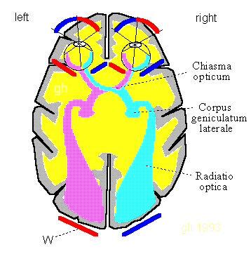
Fig.10.1: Wave fronts in the optical nervous system. Coincidentally, the orientation of projection surfaces W (red and blue) shows known projection locations. Source: [NI93] Kap.12, p.247
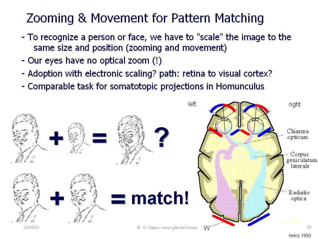
Fig.10.2: The eye does not provide any zoom function. All that remains is the "Corpus geniclatum laterale" as a cortical image projector. Sources: Israel-lectures, 2005, (Link) and [NI93] Kap.12, p.247
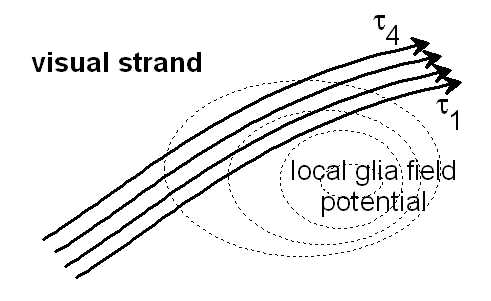
Figure 10.3: Different delay times τ1 ... τ4 can occur under the influence of a local glial field, which could lead to zooming and movement effects in the visual strand. See also IWINAC 2005, Fig.7, (Link)
It would be an indication of a projecting interference system. A recording of the real delay structure could be used to calculate the specifics of the projection space.
But is it conceivable that the delay times are directly controlled by neurons in the Corpus geniculatum laterale? It is unlikely. Neurons don't change their delay time.
The mirror-image projection of the optical system can actually only be understood using interferential approaches. The wavelength of the nerve impulses in the visual cortex is about 0.1 millimeters, the segmentation of the VC is of the same order of magnitude. See further details below [NI93], Chapter 5, p.114
If we try to switch the view between two different objects on the table, the relative position of both objects on the retina will be the same after the object is in focus.
In order to be able to perceive both objects separately, it is necessary to create a world model in the cortex in which both objects are locally represented differently (e.g. next to each other).
The shifting of the map, shown under Movement, when the delay of the channels varies, can help to solve this problem. The necessary delay variation could, for example, be obtained from a control voltage (see level generation) of the eye muscles.
The lateral geniculate body (corpus geniculatum laterale) seems to play here the role of a spatial image projector into the visual cortex.
The same idea as with the Homunculus applies to the eyes: they also "take the images with them when the eye muscles move". But here the effect is desired - like a projector, the eyes shine into a different zone of the visual cortex depending on the viewing angle. When the eye muscles directly control the glia, the image moves (movement).
Since the eyes never rest, interference integrals in the visual cortex create an "image" of the environment that is significantly larger than the part that the eyes focus on at a single point in time. This explains our modeling of the world: we always know what is going on around us, even though fixed eyes would only see a tiny area of the environment.
If the radiato optica also has lateral extensions that cannot correspond to the wavefront direction shown, then this is a sure indication that movements in the image field can be detected with it.
Because the wave front directions there are almost perpendicular to the "projection wall", these areas should not receive any image projections. But what role could they have?
In Chapter 5, p.99 of [NI93] we find a possible answer. They could detect faster movements outside of the field of vision!
However, it would be expected that the VC would then be more extensive than shown here.
Wherever we find mirrored maps in the nervous system, a projecting interference system is or was at work to form these maps.
It seems, that the interference approach offers opportunities to analyze our nervous system in all directions:
"The world is knowable!"
11. Diseases of the nervous system
One result of the theoretical investigations on interference networks would be, that neuronal communication is disturbed not only by cutting a nerve, but also by parametric fluctuations in transit time or refractoriness or by changing, for example, the length of a nerve. For example, surgically suturing a nerve together will only make sense if the transit times of individual pathways remain unchanged relative to one another, because only then can neuronal projections be preserved.
Another result would be the realization that tiny, parametric fluctuations in conduction velocity are sufficient to zoom, move, delete or overexpose neural images (interference overflow). Tunnel vision can result, for example, from small fluctuations in the conduction velocity between the eye and the VC (see zooming). Drugs that change conduction velocity or refractory period disrupt the nervous communication system because sources and targets can no longer communicate precisely with each other.
Drastic changes in conduction velocity, e.g. due to demyelination (multiple sclerosis), can only lead to communication failurs, if the nervous system can be understood as an interference network.
12. Increased sensitivity of the hand
The sharpness of a projection varies, as the distance changes. The flatter the waves are, the blurrier the image becomes. The sharpest image occurs on the smallest distance, see a simulation of the effect here.
Apparently evolution also came to this conclusion. If we look at the hand, we notice that the Nervus ulnaris und Nervus medianus are redirected over the so-called arch and then lead back up again.
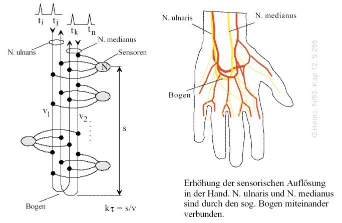
Fig.11: Opposite fibers of the N. ulnaris und N. medianus ensure, that in the hand highest sharpness and sensitivity is achieved. For details see [NI93] Chapter 12, p.255
There can only be one purpose for this amazing arrangement. We all know, that our sensitivity is highest in our hands, where we can detect touches in the millimeter range.
Rope ladder nervous system seen as interference network.
With slow and very slow conduction speed, nerve fibers open up the possibility of carrying out seemingly complex functions using the simplest means.
From the anatomy of earthworm we know, that it has a rudimentary rope ladder nervous system. It consists of paired pathways that run along the body axis and are connected transversely to the body axis via commissures. Other insects also have a more or less clearly recognizable rope ladder nervous system, such as arthropods and tardigrades.
Assuming that the rope ladder contains nerve fibers that conduct quite slowly, the meandering movement can be modeled as an interference network.
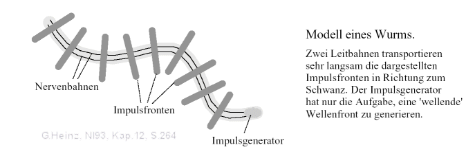
Fig.12: An undulating wave front causes the worm to meander. Source: [NI93] Kap. 12, p.264
But how can the worm meander? What role does the rope ladder play in this?
At the beginning there is the special anatomy of this nervous system. What relationship does it have to its function? Can we see an interference network in this?
It is known, that the pharyngeal ganglia located at the beginning of the rope ladder (ganglia pharyngealis superior; OSL and OSR in Fig.13) control the rope ladder nervous system. But how?
If we assume, that the left upper pharyngeal ganglion (OSL) sends out an impulse (or a sequence of impulses), then this continues along the left part of the rope ladder via GL1, GL2 and the following ganglia, see Figure 13.
However, it also arrives with a time delay in the right superior pharyngeal ganglion (OSR) and now also runs along the right part of the rope ladder via GR1, GR2 and followers, but delayed.
Assuming the same delay times T1 and T2, the partial waves meet again one after the other in all right ganglia (GR1, GR2 ...). A higher threshold value inevitably arises there. And the ganglia GR1, GR2 can stimulate the relevant muscles MR1, MR2 one after the other.
In Figure 13 we see the frozen state when the partial pulses T1 and T2 meet at the GR2 ganglion at the same time. The muscle MR2 is currently being stimulated (orange).
We abstract a slanted wavefront (WF), starting on the left side of the worm. This wavefront stimulates the muscles on the right side.
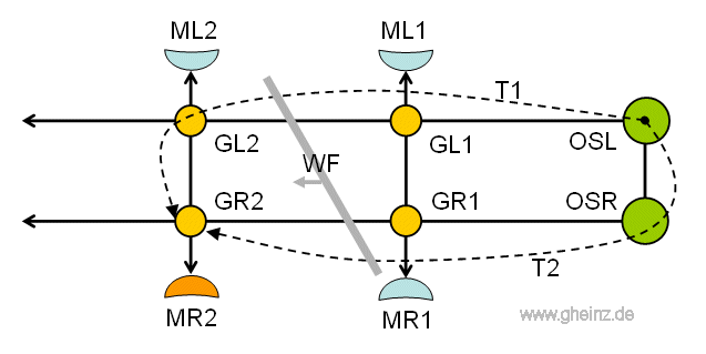
Figure 13: Rope ladder nervous system as an interference network. Here the GR2 ganglion with the MR2 muscle is being excited when both pulse wave parts T1 and T2 arrive from the left superior pharyngeal ganglion OSL at the same time. See details in [NI93] Chapter 12, p.264
We assume that the commissures, i.e. the right-left connections of the rope ladder, each have the same delay time.
We also assume that the rope ladder is constructed symmetrically, i.e. that the delay times of the sections on both sides do not differ.
Ultimately, it is also necessary that the ganglia, once excited, can activate the muscles with long-lasting potentials.
If we look at the second, right ganglion (GR2) in the picture, it becomes clear that it is excited higher when a pulse coming from T1 and a pulse coming from T2 arrive at the same time. This is exactly when the highest probability of stimulation of the ganglion occurs (orange).
Ultimately, this excitement jumps from muscle to muscle on the right side, triggering a contraction to the right side of the worm.
By analogy, a pulse or group of pulses from the OSR on the right side triggers backward excitation of the muscles on the left side.
If OSL and OSR become active one after the other, our worm begins to meander.
If OSL and OSR are activated very quickly one after the other or at the same time, the muscles on the right and left are tensed almost simultaneously and the worm contracts.
However, this only works if the commisure tracts consist of opposing monodirectional fibers instead of bidirectional fibers, otherwise there would be refractive pulse cancellation, see [NI93] Chapter 6, p.144.
Now we can read in the german Wikipedia, that the rope ladder of the earthworm is thin. It is concentrated on the abdomen side from the fourth head segment to the tail segment, the control ganglia OSL, OSR are located in the third segment.
That may be confusing at first. Why did evolution come up with this solution?
If we think of the thumb experiment, then there is a suspicion. In the thumb experiment, a change of the delays was observed as a result of a stretching/compression of the nerve fibers.
If the fibers of the rope ladder of the earthworm would be on the left and on the right side, there would also be severe extensions and compressions of the nerve fibers due to the meandring movement. As a result, it comes to opposite changes in the delays of the left and right fibres.
Apparently, the evolution decided to use constant delay times on both sides by minimizing the lengths of the links between right and left of the rope ladder.
We realize, that what appears to be quite complex behavior can be reduced to simple circuits. It is probably the simplest interference network observed in the animal kingdom. Experts should be able to measure and to verify the hypothetically introduced, relative delay times.
Flying insects also have an segmented body, the ganglia of the rope ladder nervous system of which can be precisely assigned to the segments. This suggests that the rope ladder also plays a crucial role here.
In a sectional view of a flying insect in Wikipedia it is noticeable, that two small strands for supplying a leg branch off from the ganglia of the leg segments. It would therefore be quite likely, that their legs would also be controlled via the rope ladder.
How could the earthworm model be expanded, to also take on the more complex control of the legs? After all, the legs do need to move forward, back, up and down?
Let's first take another look at the earthworm's time functions.
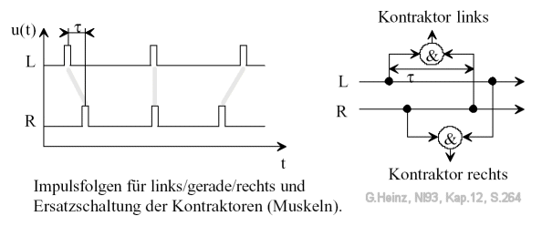
Figure 13.2: Time functions and ganglia in the earthworm's rope ladder nervous system. An opposite sign of the delay τ leads to the other side being activated. The &-characters here are intended to represent a multiplicative link type. "Kontraktor links" is intended to represent the left ganglion GL, "Kontraktor rechts" is intended to represent the right ganglion GR. Image source: [NI93] Chapter 12, p.264
The principle of the earthworm can be seen in Figure 14. A left or right "contractor" is triggered when the transit time difference τ exactly matches the incoming pulse delays.
How can the circuit be expanded to include leg control in insects?
If two different transit time differences (or wavefronts) per side are detectable in a ganglion, which differ slightly from each other, it would be possible to control one or the other detector (of the leg), Figure 15.
Of course, the connection between OSL and OSR would also have to be made twice in order to generate the two different wave fronts.
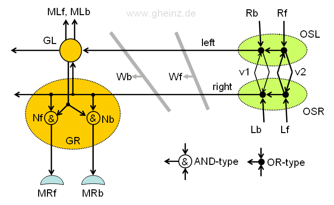
Fig.13.3: Rope ladder nervous system of a flying insect. The Leg ganglion GR and the signal generator OSL, OSR in detail. If the wave fronts Wb and Wf differ slightly, two different detectors can be used for the forward/back movement of the leg muscles control MRf, MRb, whose connection on the rope ladder varies slightly. GL, GR: ganglia for left/right legs; OSL, OSR: Left/right subpharyngeal control ganglia; v1, v2: nerve velocities; Nf, Nb detektor neurons.
The leg could then be moved independently forwards or backwards. To do this, the ganglion in question would only have to be expanded to include a second detector circuit for each side (for the left and the right side).
About the AND- and OR-neurons: Two different types are adopted. The AND type should be multiplicative in nature, where pulse peaks are needed at all inputs at the same time, so that the neuron pulses. Type OR is intended to forward every pulse at an input to the output(s). (As in Figure 14, Figure 15 also shows a double connection of the GR and GL ganglia, which is also used in the earthworm to prevent refractive extinction of pulses running against each other.)
Pulse generator OSL, OSR: As can be seen, the pulse generator on both sides would have to be designed twice, for forwards (index f) and for backwards (index b). Signal feedback between OSL and OSR with self-excitation is not to be feared, if the refractory phase of the OR-type neurons is high enough.
About the function of the pulse generator: Two different conduction speeds v1 and v2 create two different delays on the commissure pathway (with the length s) between OSL and OSR, with τ1 = s/v1 and τ2 = s/v2. We assume, that v1 < v2 is. The interconnects v1 are therefore shown thinner than those for v2. If a forward pulse arrives at Rf, v1 is activated and generates a wave front Wf, similarly a backward pulse is generated at Rb over v2 with a wave front Wb.
Detectors GR, GL: A first detector neuron Nb would detect the wave front Wb and activate the leg-go-back muscle MRb, a second detector neuron MRf would detect wavefront Wf and activate the leg-forwards muscle MRf.
The detector pair Nb, Nf can in principle be identical. It would only be necessary to select the connections of the pair of detectors on the rope ladder slightly differently.
A particular property of this circuit should be mentioned, which can be observed at insects. As with an earthworm, the pulses continue to the back part of the insect. They excite subsequent ganglia on this side. Each leg receives the same command with a slight delay: go forward or go backwards. Thus the movement of the pairs of legs between each other is automatically coordinated!
If the leg is additionally to be moved up or down, two additional detectors per leg would be necessary. Or the up/down movement is coupled with the forward/backward movement. The leg rises forward and lowers backwards (although this would have the disadvantage that the animal would not be able to walk backwards). But here it becomes speculative; microscopic analyzes and detailed studies of the behavior of a specific animal species would be required.
Elsewhere on this pages it is written about interference networks: "The form encodes the behavior". It seems that this sentence is also valid here.
It never ceases to amaze me what brilliantly simple constructions nature has devised for behavior that appears so complex!
In the book "Neural Interference" from 1993 (NI93), circuits for sequence analysis with delay lines were developed in Chapter 8b, see p. 181 (Figure 14.2).
If we consider the complex and precise movements of a farmer mowing a meadow with a scythe, or of a dancer, but also everyday activities such as climbing stairs, noises and sound recognition, or, last but not least, word recognition and, in their hierarchy, sentence recognition, etc., analyzers that can recognize and analyze sequences are always required. How can we imagine such neural circuits in their simplest form?
We assume that a time function to be analyzed here arrives pulse-density modulated. High amplitudes are converted into pulses.

Figure 14.1: Example pulse conversion of a noise, a sound, or a word (symbolic). If we detect positive and negative maxima, we obtain a pulse sequence that characterizes some features of this sequence.

Figure 14.2: Excerpt from NI93, p. 181. On the left, a runtime representation; on the right, a signal-theoretical node abstraction as an FIR filter. The input is a pulse sequence x(t), the output y(t) is a pulse, wi are weights. q may be a pulse shaper.
Quote: "The basic idea is that a code, which can be scanned in multiples of τ, is delayed along a circular path, with the neuron at its center. Each tap on the circle has the same distance from and the same travel time to the center, so that the travel time on the radials is compensated. The taps leading to the center are arranged on the circle in multiples of τ. Stimulating and inhibiting weights wi on the neuron can be selected so that excitation only occurs with the correct code. At least n pulses are required to trigger the detector once. n is the number of inputs to the neuron."
With this arrangement, it would already be possible to detect periodic time functions (sounds). With several neurons connected in this way, the auditory spectrum could be spectrally decomposed (for Fourier analysis with different τ).
But how can a sound or a word be recognized in the simplest way?
The answer can be found on page 188 (NI93, Chapter 8b). To do this, the circuit's weights must be modified according to the pulse sequence to be filtered out, see Figure 14.3.

Figure 14.3: Sequence analyzers. Excerpt from NI93, p. 189. On the left is a radial sequence analyzer, on the right is an axial variant. Here, the highly valued weights are shown in gray, and the unneeded weights are shown in black. The notation of inputs in curly brackets is to be read from right to left; black means 0, gray means 1.
If we now imagine away the signal-theoretical abstraction of a sampling rate with τ, which does not occur in nature, then we have arrived in reality. It is sufficient to tell neuron n via another, generalizing input (bias) that it should increase the weights of the sound, noise, word, movement, or behavior (generally a sequence) that has just arrived. How nature tells the neuron to adopt the weights remains to be seen. One thing, however, is clear: In order to learn something, a triggering stimulus (entered here as bias) is always necessary, which tells the neuron to increase relevant weights and reduce irrelevant ones in order to continue the learning process. The triggering stimulus could be the clinking of a falling glass, a stumble, an accident, an observation (aha! moment), or whatever.
It should be noted that a one-time, complete transfer of the weights would not lead to success. In the next comparable situation, the time function to be detected (training data) will generally deviate significantly. Nature will therefore have to learn slowly to gradually adjust the weights. It should also be noted that weights must be both increased and decreased to avoid the risk of all weights being at their limit one day.
If we observe a nerve fiber bundle with fibers of different conduction velocities converging on a neuron (Figure 14.3, right), we have a second type of sequence analyzer. This form is probably found millions of times in the cerebral cortex. See, for example, a Golgi preparation by Ramón y Cajal in the Eccles in Figure 12, p. 20.
If we compare the arrangement in Figure 14.3 (left) with a technical implementation as an FIR filter in Figure 14.2 (right), it becomes clear how far biology still leads technology in terms of development. While biology gets by with one or two neurons that are micrometers in size and consume nanowatts, a corresponding technical implementation requires a thousand times more power dissipation, size and weight.
What we need to reach this efficiency class of biology, are analog delay networks as interference networks of a technical nature. The basic prerequisite for this would be simplest delay lines of an analog nature. Now we know that these already exist; think of polysilicon conductors on integrated circuits. However, these are still millions of times faster than nerve fibers, so they are still very fast. This could be an advantage when we consider ultrafast computer science, whose 'neurons' pulse in picoseconds. In my opinion, there is a field here that is definitely worthy of funding. Individual companies would likely have difficulties meeting the financial requirements.
It is not granted to any mortal to recognize life in the dispersal of physical or chemical substance, in diffuse, if you will, spiritual form, and if that would happen, it would certainly be the hardest blow to the modern scientific outlook could.Rudolf Virchow
© Copyrights for this page: Images can be used without restriction, if the name of the author and the origin of the image are visibly noted as the web address of this page.
Translated using Googles beautiful translator. With corrections.
File created sept. 30, 1995. Continued editions.
Visitors since Dec. 2021: